In a post where I talked about modelling data in graphs, I stated that graphs can be used to model different domains, and discover connections. In this post, we’ll do an exercise in using multi-domain graphs to find relationships across them.
An institution can have data from multiple sources, in different formats, with different structure and information. Some of that data, though, can be related. For example, we can have public data on civil marriages, employment records, and land/property ownership titles. What these data sets would have in common is the identity of individuals in our society, assuming of course, they were from the same locality or country. In these scenarios, in order to run a cross-domain analysis we need to find ways to connect the data in a meaningful way, to uncover new information, or discover relationships. We could do that to answer questions like “What percent of the married people own property vs those that don’t”, or more interestingly “who is recently married, and bought property near area X while changing jobs”.
In this post, we’re going to explore that kind of scenario. We’ll make use of randomly generated flight, call, and employment data. To bind them together, we’re going to come up with a little use case to help us. As with any problem, there are several ways in which we can solve them. In choosing an approach, one of the first we need to do is to pick a data store that can aid in our querying.
On the hand, we have relational stores are very good for relational data, and transaction processing. Then, we have key-value stores, for easy retrieval of uniquely identified entities; they can be rather fast when they operate in memory. Document stores are similar to key-value stores, but can host more complex objects, while column stores are the equivalent of relational ones, but process data in a more ‘vertical’/column oriented manner. And then, there are graph stores. Among these data stores, graph databases are the ones that are designed primarily for relationships, and hence, the ones we will be using in this example. It is far from my intention to imply that relational, document, column or any other type of store is not suitable for this kind of problem. Different data stores can be applied to different problem domains by people, depending on their circumstances. Personally though, I see graph stores as the path of least resistance for this particular problem. We will begin with our cover story, and then we will take a look at our data and data models, before we begin our inquisition on the data sets.
The Story
A company, WT Enterprises, is working on a secret R&D project to develop the next generation solar powered generators, and its managers suspect that one of its employees is selling their trade secrets to a competitor. They suspect that Enterprise XYZ, one of their direct competitors, is somehow gaining insight into their work to come up with competing products.
As of now, we’re contractors for the Interpol, and our job is to investigate this trade secret violation allegation.
We will start by asking some simple questions on each data set, just to refresh on minds on how to query data in Neo4j, and then we’ll try and use all three data sets, gradually, to find our potential persons of interest (POI). The idea is to see how we can have different domains in the same graph, and find connections in the data.
You can get the source code for this tutorial on github. I used python for this example.
The Data
We have 3 randomly generated data sets: flights, calls, and employment records. If you use the source code to generate the data, it will change every time to run the code, since, you know, it’s random; for this reason, we need to seed some specific events, like flights and calls, so that we can be sure we get the results we seek. When you run the seed.py script, it generates 4 random 4 sets of data, i.e. people, calls, flights, employment, and dumps them out to JSON files. You can use those files to import the data using some other programming language/framework, or data store. To alter the amount of data generated, just modify the N dictionary/map in the seed.py script. In terms of structure, the data sets are pretty simple.
People
Calls
Flights
Employment
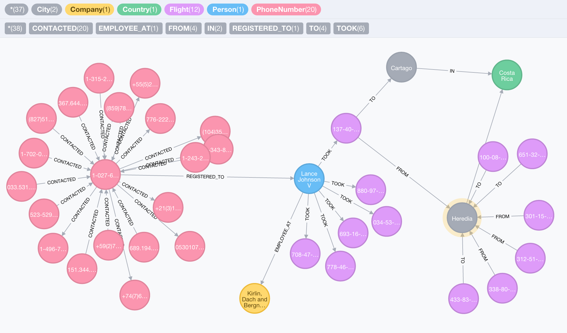
All flights, and phone calls in our generated data sets occurred in the year of 2014. You can see the visualisation of some sample data here
The Graph Model
The graph model for our problem spans all three domains:
- (:
PhoneNumber)-[:REGISTERED_TO]->(:Person) - (:
PhoneNumber)-[:CONTACTED {weekday, hour, timestamp}]->(:PhoneNumber) - (:
Person)-[:EMPLOYEE_AT {since, until}]->(:Company) - (:
Person)-[:TOOK]-(:Flight{timestamp}) - (:
Flight)-[:FROM]->(:City) - (:
Flight)-[:TO]->(:City) - (:
City)-[:IN]->(:Country)
To keep the model simple, for this demo, we ignore certain particularities in each domain, e.g. the change of phone number ownership from one person to another is not addressed in this model. Visually, we get the following:
The Data Inquisition
I have covered how we can query graph databases before, in a quest to identify caveats of graph models. This time though, we’re going to concentrate on identifying connections, in the form of graph paths, using the multi-domain data model we have.
Basics
We will start off by asking some trivial questions, just to refresh our understanding of querying graphs. To do that, we will ask the following 2 questions:
-
Who are the people that took the most number of flights to any destination between the months of January and June 2014
-
Who are the people that took the most number of flights to any destination for each of the months between January and August 2014
The two questions are very similar. The only difference between them is that in the first, we are interested in a person vs number of flights relationship for a period of 6 months, i.e. January to June 2014, while in the second we want to split those entries by month. Let’s start with the first:
Q1, query:
Running Q1 with count equal to 1, and limit set to 10 on with a randomly generate data set, I obtain the following results:
| Person | No. Flights | Destination |
|---|---|---|
| Loyal Keebler | 3 | United Kingdom |
| Shanon Jerde | 3 | United Kingdom |
| Heidy Fay | 3 | United Kingdom |
| Veda Lubowitz | 3 | Slovenia |
| Antonina Berge | 3 | Slovenia |
| Lindsey Howe IV | 3 | United Kingdom |
| Michel Schuppe | 3 | United Kingdom |
| Collin Langosh | 3 | Slovenia |
| Milissa Cassin | 3 | Slovenia |
| Guido O’Hara | 3 | United Kingdom |
The table gives the name of each person, the total number of flights they took to each destination, sorted by the number of flights. Our seeder seems to a have suspicious lean for the UK and Slovenia. Remember, we scoped our query to flights that took place between to January and June 2014. The result is straightforward, so let’s move on the second part. We have queried the data for entire period, and now we want to split the results by month.
Q2, query:
The Cypher query is very similar to the first. In fact, they are almost the same. We only exclude the limitation on the number of results we want to see. To divide our results by months, we have to run the same query with different startDate and endDate parameters. Using Neo4j’s transactional endpoint, we can send a batch of these queries at once, and retrieve their results. You may refer to the source code to see how to do this in Python, with the neo4jrestclient. I ran the query with count set to 1, and the result set that I got looked like this:
Between 2014-07-02 and 2014-08-01
| Person | No. Flights | Destination |
|---|---|---|
| Nunzio Funk IV | 2 | Latvia |
| Miss Janiya Erdman PhD | 2 | Slovenia |
| Karan McLaughlin | 2 | United Kingdom |
| Mr. Jett Connelly Jr. | 2 | Japan |
| Chancy Pagac | 2 | United Kingdom |
| Dr. Fount Marquardt IV | 2 | Turkey |
Between 2014-08-01 and 2014-08-31
| Person | No. Flights | Destination |
|---|---|---|
| Mr. Eliot Luettgen PhD | 2 | Japan |
| Courtney Mueller | 2 | Thailand |
The two sets are for the months of August, and July. I used a 30 day interval moving backward, which is why the result for July starts on July 2nd.
I will just call out the reader’s attention to one aspect here: Grouping. Notice that we don’t have an explicit GROUP BY statement in our query. Instead, we just return the person’s name, a count of the number of flights, followed by the destination. Based on our relationships, Cypher automatically groups the count of the number of flights by the destination for each person. In other words, we group data in our return statement. Related nodes are filtered in our result based on the other entities we return along with them; so because each person has several flights, to different destination, Cypher will group our country based on each pair of (Person, Destination).
Person of Interest
Now that we have, hopefully, refreshed our memory on how we can query data, we can proceed to try and solve our original problem. First of all, our investigators tell us that our person of interest might be contacting the representative of Enterprise XYZ on a fixed schedule, i.e. Wednesdays, between 6pm and 10pm. We’re gonna use that as a starting point, and build a query that will, gradually, get us close to our potential persons of interest, and we’ll do it in 3 steps:
-
Find phone numbers that have made calls to the representative of Enterprise XYZ, on Wednesdays, between 6pm and 10pm
-
Among the people that called the representative, find those that have flown in or out of one of Enterprise XYZ’s offices in Japan, or the UK
-
Among the people that called the representative, and flew in or out of one of Enterprise XYZ’s subsidiaries, find those that have an employment history at WT Enterprises’
Let’s get started.
Step 1: Callers
A glance at our data, and model, and we can tell that finding numbers that called the representative at a certain hour, and weekday a is fairly trivial task:
We query for numbers that made the call on a Wednesday, between 6pm and 10pm, and retrieve the names of the callers, as subjectName, and number of calls they made in at that weekday/hour, as numberOfCalls
With my dataset, the results look like this:
| Subject Name | No. of Calls |
|---|---|
| Dr. Lorelei Smitham | 4 |
| Kiran Trope | 17 |
| Mr. Tyrone Gislason PhD | 1 |
| Brittni Aufderhar | 9 |
| Autumn Kassulke | 3 |
Kiran Trope and Brittni Aufderhar both stand out from this list, as the two have contacted the representative on a Wednesday, after work hours, on more than five occasions. But that’s hardly enough for us. Any of those people could be a friend or a person with whom he is business with. What we need to do is to narrow our search further to get more plausible information; we’re going to do that by taking this list,and finding who among those names has flown in or out of one of Enterprise XYZ’s offices, if any.
Step 2: Flights
Enterprise XYZ several offices spread across two countries, the United Kingdom and Japan. Our task is see if any of the names from our previous result has flown to either one of those two countries over the year of 2014. We start with our query:
The query builds on our previous one, except, instead of returning the subject names and number of times they called, we use the subject and check if they have taken any flights to either the UK or Japan, the countries variable in the query. The result set consists of the person’s name, ID, name of the country they flew to as well as the number of times they flew:
| Name | Person ID | Destination | No. flights |
|---|---|---|---|
| Mr. Tyrone Gislason PhD | d54fbbdf-… | Japan | 1 |
| Dr. Lorelei Smitham | 994f4117-… | Japan | 1 |
| Kiran Trope | 05382319-… | Japan | 3 |
We have narrowed list of potential persons of interest from 5 to 3. Tyrone, Lorelei and Kiran are the only 3 people who have spoken to the representative, and have flown to an country where Enterprise XYZ has an office. Despite being better than what we got from step 1, this information is still not enough for us to make strong connection. All 3 of these people could be business partners, or even colleagues for the representative of Enterprise XYZ under investigation; we’re going to have to take another step in finding stronger circumstantial evidence.
Step 3: Missing Link
Our last query gave us 3 potential persons of interest; so far though, all our links are not substantial enough to support investigating any of the three individuals: a phone call and a flight are hardly enough to connect these people to the representative in a meaningful way. So, we’re going to turn to our third data set to find the missing link: employment records.
The task is simple: find out if any of the potential person’s of interest has an employment record at WT Enterprises. The premise here is that if a person has been working at WT Enterprises, has a history of contacting the representative of Enterprise XYZ, and they have flown to any country where one of his company’s office might be, that should give us plausible enough evidence to pursue as a lead.
Final query:
Just like before, we build on the previous query; instead of returning the results, we use the potential POIs and see if any of them were employed at WT Enterprises in the beginning of the year 2014, when they began they solar powered generator project. The result set consists of the person’s name, ID, the date in which their employment commenced, and the day it ended, if they no longer work at WT Enterprises:
Result:
| Name | Person ID | Employment Start | Employment End |
|---|---|---|---|
| Kiran Trope | 05382319-… | 2013-07-01 | 2014-09-30 |
And voila. We have found our POI. It seems that Kiran Trope is our most likely suspect, as intended, since we seeded the database that way. She worked at WT Enterprises between July 2013 and September 2014, a time during which she had access to acquire intel on WT Enterprise’s projects. She has been in contact with a person working for WT Enterprise’s direct competitor, whom she called 17 times over the period of a year; and, she also flew to Japan on at least 3 occasions, where she could have delivered trade secrets on WT’s solar generator projects to one or several of Enterprise XYZ’s offices. And that’s it. Our part is done. Now, back to the real world.
Final Thoughts
In this post we saw how we can use a graph database to find connections in data from multiple domains. Our cover story gave us three different data sets to work with, and connect, i.e. flight, call, and employment records.
Our main goal was to see how we can perform cross-domain data querying efficiently in a graph database; moreover, the mechanism for finding connected data were shown to be relatively straightforward, as there were steps of processing in our code; everything was done directly with the database. You can explore the data domain, and think of new ways to extract information as a fun exercise. Obviously, our findings may not that interesting because we’re using randomly generated data, but the ideas are useful for real data sets as well.
As a side note, all queries ran in under 300ms the first time, and under 100ms on the second run, once their execution paths were cached by the database. You can populate your database with more data, and run speed tests to see how it performs. This just shows are efficient graphs can be for making connections, even in densely populated data stores.
Our assessment could have also been performed visually, with the help of a graph visualization tool, or Neo4j’s own Web Admin Console, if you would like. Note that there are complex systems that allow you to perform this kind of querying across data from different data stores, e.g. logs and SQL data stores. If your use case is a relatively simple though, you can probably make do with a solution similar to the one we implemented here.