In this post I describe a framework and experiment in simulating context-free bandits

The explore-exploit dilemma can be found in many aspects of every day life. To put this in concrete terms, imagine a person receives a free 30 meal gift card from a new breakfast restaurant that just opened up in their city. The restaurant may be well known for having good breakfast options; and as a breakfast lover, the person wants to find the best breakfast option on the menu — note that best here means personally favored, not categorically best, as in defined by a food critic or social media popularity. There are dozens of breakfast options, yet, not all of them are equally good, as per the person’s preferences. The resource constraint here is number of meals, which in this case is limited to 30. Assuming a limit of a single meal per day, that gives 30 days as slots to try out the meals. The goal is to maximize total reward by spending as many free meals as possible on the most favored menu option. For instance, if the person tries menu item four, and really enjoys it, then the reward can be 1. If they don’t, then reward can be 0 - this is the lost opportunity in getting a positive experience, which is also called regret.

Issues with this type of problems should be evident by now; let’s pay attention to two of them in particular: (1) from the get-go, the person does not yet know which of the options on the menu will be their favorite, since they haven’t tried any of them; and (2) there is a limited number of meals to be had. The greatest known regret would come from finding the favorite option on the very last day, because the person would only get to spend one meal on it. I say known because, granted a second gift card or just by visiting the restaurant at their own cost, there is a possibility of actually having a menu option that is more favored over all the previously tried ones. Hence, there is also an unknown or hidden regret for the person.

The best case scenario, on the other hand, would be the person having the most favored menu option first - which is practically impossible without actually trying out the other ones, since there would be no way to know if there is a breakfast option that is more favored without comparing them. Decisions. Decision. Decisions.

This is the explore-exploit dilemma. There is a need to explore as many options as possible to find the most favored one - yet, one would also like to exploit the ones known to be highly favored. With all of these variables in hand, wouldn’t it be good to understand how a person’s journey might go? What the best and worst case scenarios are? This is where simulations come in handy. In an earlier post, I described how I simulated the Monty Hall problem to work out the dynamics of probabilities of the game show. This time around, I implemented some of the algorithms from the Bandit Algorithms for Website Optimization book in a simulation framework for context-free bandits, with a few modifications, to adjust for certain aspects of common real-life problems. Running simulations on the framework has given me the following benefits:

• Getting expectations of performance of different decision routes
• Estimate number of steps to reach stability and become familiar with uncertainty — when can a winner be called out?
• Have fun visualizing different behavior!

Note that this choice problem, the breakfast gift card, is a very simplified representation of a real problem. There is far more complexity in this, like the fact that rewards here are assumed to be fixed, whereas best is more of a ranking that changes over time, and can depend on other aspects like the state of the ingredients used on a given period. I leave that aside for now to focus on the concepts under consideration.

Principle

One can think of multi-armed bandits as a framework for learning. There are different algorithms in the wild for them. One of the most common ones is known as epsilon-greedy, and it works like this:

epsilon = 0.1 # probability of exploration 
actions = ['cafe-la-plaza', 'cafe-la-playa', 'cafe-central']
steps = 30
bandit = CleverBanditAlgorithm()

for i in range(steps):
	r = random.randn()
	if (r < epsilon):
		a = bandit.pick_at_random(actions) # pull action
	else:
		a = bandit.best_action_so_far(actions)
	
	reward = take_action(a)
	bandit.update(a, reward)

At the highest level, a multi-armed bandit does two things: (1) explore alternative options to estimate expected reward, i.e. how good an action is; and (2) exploit the best actions to maximize total rewards. The way in which they decide when to explore or exploit is one of the major differences between the various algorithms. For epsilon-greedy, for example, there is a fixed probability of exploration that’s defined at the beginning. In the code snippet above, it’s set to 10%. That means that on any given chance to pick an option, there is a 10% chance that an option will be chosen for the purpose of exploration. More specifically, for epsilon-greedy, that decision is made completely at random. So, if there are 20 menu options in the restaurant, and exploration is set to happen in 10% of the cases, each menu option will have equal probability of being chosen at random on three different occasions — 30 free meals x 10% exploration = 3 meals for exploration. The action of making a choice is also called arm-pulling. Reasons for this are obvious once we understand the origin of the name multi-armed bandits.

Now we can start looking at the modules that make the optimization framework, BOE: bandit observation engine. Clever name for a clever tool.

BOE

There are a few key modules I chose for the design of BOE to reflect the view portrayed here of the nature of the problems bandit algorithms address: the environment, the oracle, the simulator and a reporting module. Let’s go through each and understand what they do.

Environment

This is a representation of the real world — sort of. A certain type of real world. When an action is taken in a bandit setting, a reward can be observed for it - this can be immediate or delayed. When a person eats a meal, they know right away whether they enjoyed it or not. But think of cases where this feedback isn’t immediate, like writing an article. A writer can spend days or even weeks writing an article, and they won’t know how it will resonate with their audience until their article is published. Delayed feedback is actually handled by the simulator module. The main aspect of feedback that the environment module deals with is the nature of the reward itself*.* Let’s expand our problem a little bit to discuss this.

A person can try a few meals at a restaurant and rank them by giving each one of them a score that is reflective to their preference. You can assume that each meal will taste the same each time it’s served; but that’s not what happens in practice. Some days the omelette is great, and some days it’s just acceptable — this may be a factor of the eggs or other ingredients used, the chef, or even what you’re drinking along side it. If so, then the score for the omelette will be a variable dependent on those factors. To simulate this, one needs to have an environment (arm) that gives rewards based on these specific conditions. Or at least, one that varies its rewards based on the time step to emulate that behavior. For the first version of BOE, I implemented the simplest of environments: a Bernoulli arm, where the reward is given by chance, based on some fixed probability p.

So for instance, the value of p is set to 0.3, then pulling an arm 100 times will give an expected total reward of roughly 30 points. For the free meal gift card problem, having a meal with an average reward of 0.7 would mean that a person enjoys seven out of every 10 servings of that same meal.

Oracle

Oracles are algorithms. As of this writing, there are three algorithms I implemented in BOE: Epsilon-Greedy, Softmax, and UCB1. Their characteristics are well described in John’s book. When they decide to explore, they pick one of the arms to explore according to their own internal policy. And when they decide to exploit, they choose what they believe to the the arm with the highest expected reward.

Somewhat similar to The Matrix, an oracle predicts the future. Unlike the matrix though, it doesn’t guess what will happen. Rather, it estimates it from past experience. For the free gift card problem, this estimation is a likelihood of preference, or more specifically, likelihood of a person enjoying a meal the restaurant. At the start of a simulation run, one can assume there is no information about any of the given arms - this would represent a person that is unfamiliar with any of the menu options. So, one can assume that the expected reward for each is the same, and that it’s equal to zero - or some other value. In BOE, it’s always zero. From that starting point, different arms will be played until, eventually, the best arm is known.

Simulator

This is the main engine. The part that is responsible for running simulations. First, it may be relevant to note here that BOE is a configuration based tool. That means that to execute a simulation in BOE, called an experiment, one specifies a configuration file, detailing the specification for that simulation. Below is a snippet of what an experiment configuration might look like:

experiments:
  - id: egreedy-explore-exploit
    algorithm:
      id: epsilon-greedy
      configs:
        - epsilon: 0.1
        - epsilon: 0.2
        - epsilon: 0.4
    arms:
      - type: bernoulli
        name: jump-back-in
        p: 0.01
        reward: -1.0
      - type: bernoulli
        name: new-releases-from-favorite
        p: 0.01
        reward: 1.0
      - type: bernoulli
        name: box-office-breakers
        p: 0.02
        reward: 1.0
      - type: bernoulli
        name: worst-movies-ever
        p: 0.05
        reward: 1.0
    config:
      report:
        ci-scaling-factor: 0.1
      simulation:
        runs: 15
        trials: 10000
        update-delay: 100
        initial-update-steps: 50
        snapshot-steps: 10

The following aspects are defined:

(1) id: this is just a name for the experiment

(2) Algorithm: the name of the algorithm — between the supported ones — along with any algorithm-specific parameters, each one specified as a map in the configs list. In the example above, three different configurations of Epsilon-Greedy are listed: one with 10%, one with 20%, and one with 40% exploration.

(3) Arms: here, the arms for the environment are specified, along with a name and any other specific parameters; right now, only Bernoulli arms are supported. Note that arms can have negative rewards (e.g. think about a person having a meal they dislike). However, for algorithmic purposes, all rewards are internally mapped to the range of zero to one for the bandits.

(4) Simulation: here, simulation specific parameters are setup, such as the time horizon of a single run, and the number of times execute a run, since it’s a Monte-Carlo simulation;

For the simulation configuration, there are three parameters that I think are worth going into a bit of detail for: update-steps, initial-update-delay, and snapshot-steps.

update-steps and initial-update-delay

In problems where bandits can be applied, such as optimizing the delivery rate of messages for users or deciding on the background of a page, there can be a delay in feedback due to several exogenous factors, such as lag time for users interacting with the content. For example, for a company that sends a newsletter every week, it can take hours or days for their consumers to interact with or take any kind of action from it. Then, there will be a waiting window to allow the response materialize, before updating the bandit. In BOE, it is possible to simulate such scenarios where the update and decisions are made with a fixed window.

Both delays parameters are defined in terms of steps, e.g. one can specify updates to happen every 500 steps; I chose this as a fair compromise because: (1) it’s consistent throughout the experiment, and (2) it gives enough flexibility to simulate a few common cases. So say a business sends 10 newsletters every day. By the end of the week, they will have 70 newsletters out. Having an update step set to 70 would be equivalent to saying that after full week’s batch of sending newsletters, the feedback from those letters is incorporated before sending out the following 70 hundred. What this misses out on is that the feedback from the last letters may not be immediate, and can in fact take days to arrive. As such, there is an assumption here that during that time no letters would be sent. BOE can be improved to account for such cases.

snapshot-steps

This is parameter is very important for the final output of a program execution - the visualization of the results. It defines how often snapshots of performance of the bandit as well as it’s knowledge should be logged. A small value means more time steps to visualize, which can help with short length experiments. A larger value means less sampling, and can be useful for long horizon experiments.

With that, the experiment is pretty much ready to be executed. There is only final module to present.

Reporting

No simulation is complete without a report. In BOE, snapshots of the bandit and experiment are recorded at pre-defined steps. Since the simulator runs several executions of the same configuration to average the results, the report is also a representation of the averaged values. Below is an example of a simulation that involves two arms: omelette and pancakes. This simulates a person that likes omelette (0.8), but enjoys pancakes even more (0.89), and it runs for 356 steps (trials).

experiments:
  - id: omelette-or-pancakes
    algorithm:
      id: epsilon-greedy
      configs:
        - epsilon: 0.5
    arms:
      - type: bernoulli
        name: omelette
        p: 0.8
        reward: 1.0
      - type: bernoulli
        name: pancake
        p: 0.89
        reward: 1.0
    config:
      report:
        ci-scaling-factor: 0.1
      simulation:
        runs: 15
        trials: 365
        initial-update-delay: 0
        update-steps: 1
        snapshot-steps: 1

Data for the final report is stored as serialized numpy arrays in a folder defined for the experiment. Along with that, BOE generates an HTML report with the metrics, that looks like the figure below.

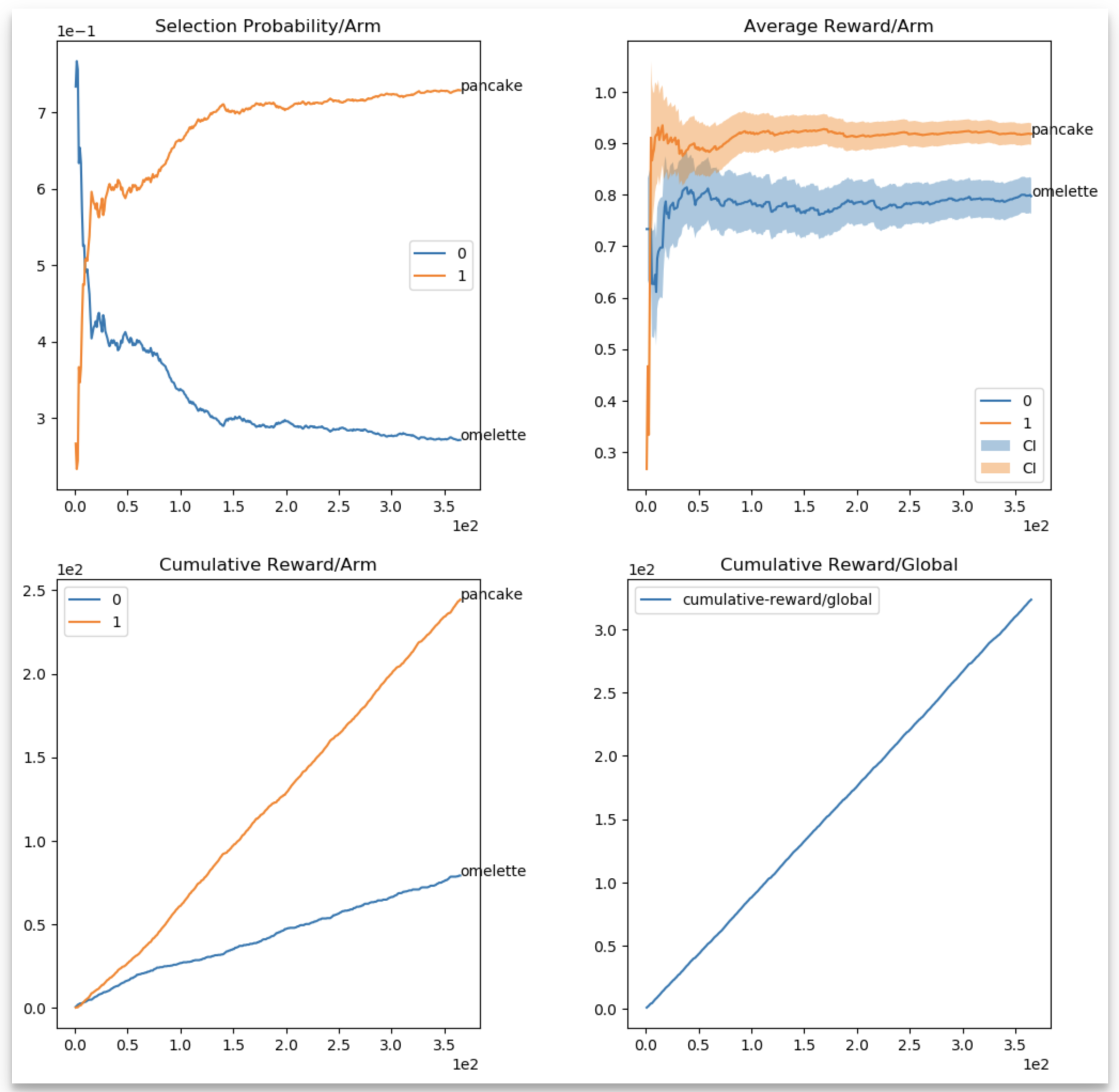
There are few noteworthy points of the report:

• There is a selection probability (top left), average reward per arm (top right), cumulative reward per arm (bottom left), and a global cumulative reward (bottom right) figure.
• For the average reward per arm, there is a confidence interval, computed using Chernoff-Hoeffding upper confidence bounds (see UCB algorithms in Lilian’s blog), scaled for visualization purposes, using the ci-scaling-factor configuration parameter — I used this as means of having uncertainty around the values, even for non UCB based algorithms; it is only for visualization purposes;
• The global cumulative reward is essentially total satisfaction measured at each snapshot step.

Running

To run experiments in BOE, it’s as easy as defining a config file and executing the experiments. There are example experiment configurations under the experiments directory, and example run scripts under the sbin directory of the repository. Start by running the pre-defined experiments, and then tweaking them to see what changes. Making modifications to the algorithms, time horizon and update interval can drastically affect total reward, as well as the time it takes to learn the “true” average rewards for the different arms.

Going Further

That was an introduction BOE, a framework for testing context-free bandits. However, there are several factors of the problem presented that merit further discussion. I’ll address three pertinent ones before wrapping up.

Prior-beliefs

One of the assumptions was that from the onset of each experiment, very little information is known about the different breakfast options due to lack of personal experience of a person with them. In practice though, people can resort to past personal experience, as well as friends and acquaintances to formulate a prior expectation i.e. a prior-belief. Having this set of prior-beliefs, the starting ground for each option may not be the same nor will it necessarily be equal to zero. And that can affect the choices made in the beginning, and ultimately the total reward.

Factoring context

One of the key aspects to any decision making is the context in which the decision is made. The price of dishes, their variety, the person’s disposition to liking variety, their sensitivity to pricing and price changes, and time of the year can all be factors that affect the ranking of breakfast menu options, i.e. the expected reward from each one. This is where contextual bandits are useful - a modified version of multi-armed bandits where the expected reward is not simply a static value, but a function of the context as well.

Dynamic rewards

Finally, tastes change, and the rewards need to be readjusted. Having a static probability p for average reward can be representative of several real-life problems; but it can also be misrepresentative of many other problems, even if that probability is tied to a context. It’s more interesting to simulate such scenarios, where seasonality or personal disposition of travelers affects their judgement in ranking options.

Conclusion

This was an introduction to BOE, a little framework I made to simulate context-free bandits to understand them better. If you feel like learning more about them, you can fork it from github and run simulations, or even add different algorithms and environments.