In this mini-series of posts, I will describe a hyper-parameter tuning experiment on the fashion-mnist dataset.

In the Part I, I described the workflow to create the data for my experiments. In this post, I describe creating the baseline and a guided hyper-parameter tuning method.

The Baseline

For any modeling tasks, I always like to create a baseline model as a starting point. Typically, this will be a relatively basic model in nature. This serves three very important purposes:

1. Establish a lower bound on performance: before applying more complex algorithms, it’s always good to know what you can get away with using basic ones - or even heuristics
2. Test the triaining and testing pipeline: in the end, a project produces artifacts, which can be models, statistics reports, charts, etc. Going from start to finish, creating all elements of a project is much easier with a simple (even low-performing) model. They typically train faster, are more predictable in terms of their behaviour, and you can see how your pipeline is working. This way, you prevent some trivial mistakes (e.g. are you exporting the actual logits or the probablities) out of the way, and you can address the more important aspects of the project, such as the right metrics to use, early on.
3. Makes iteration faster: having a code base with all the components ready to go makes it easier to start modifying how you do things, e.g. changing the model, alterting the data processing logic, adding or removing metrics.

The dataset for this project, fashion-mnist, is an image dataset. Since I was using tensorflow, and testing out tensorflow 2.0, I chose to use a fully connected neural network as a baseline. That way, most the plumbing around it would remain relatively the same.

Side: This time I could have actually done training on the cloud - and I did, for some parts - but I decided to put my GPU to work. I had an NVIDIA RTX card, running on Ubuntu, and getting the right version of tensorflow, nvidia-drivers, CUDA and cuDNN library aligned was a song of ice and fire in itself. Still, it was worth it to be able to train locally, with full visibility of the hardware monitoring. It’s been a while.

Hyperopt

My intention was to be able to run hyper-parameter tuning on a model. To that end, I needed two things: (1) a model and (2) a way to run hyper-parameter tuning. The first one was easy: a fully connected network would do the trick. Now, onto the second aspect.

The most rudimentary way of running hyper-parameter tuning is to run a grid search. Basically, you devise all the possible values for each parameter, build a set of their combinations, and train with each. In the end, you pick the parameters that give you the best performance on your validation set. This, naturally, can be a fairly computationally expensive process.

So, I wanted a library that offered a guided solution, and was convient for using with my existing code, with mild changes only. As with many other data science aspects, there is a world of options available for hyper-parameter tuning. Particually, in python. I found tools such as tune, bayesian-optimization package, AX from facebook and hyperopt. They all pretty much provided what I needed. I chose to try out hyperopt because I liked how you could express priors about each paramater in different ways. And, it had a distributed option, which I wanted to test out. Let’s dig a little into the library and algorithms.

The Approach

Hyperopt is library described in a paper titled Making a Science of Model Search: Hyperparameter Optimization in Hundreds of Dimensions for Vision Architectures (2013), so you can tell what the authors intended. It uses an approach to optimization called Sequential Model-Based Global Optimization (SMBO).

SMBO is an active learning problem solving approach. Essentially, it tries to learn a function that can minimize our objective - in this case, our objective is a better learning algorithm, and so the loss can be the negative classification accuracy, for instance. One of the algorithms the library implements to achieve this is the Tree-Parzen Estimator (TPE), which is described in Algorithms for Hyper-Parameter Optimization (2011).

TPE is an interesting approach to hyper-parameter optimization. Without going into many details, the algorithms does the following:

• The parameter space is defined as a tree partitioned space, e.g. the number of neuros on layer 3 (leaf parameter) is a leaf node of the branches of the space where the network has more than 2 layers (parent parameter).
• Once partitioned, each parameter is defined according to a prior distribution.
• Then, the model learns the probabilities p(x|y) and p(y) to determine the best parameters x (hyper-parameters) that maximize it’s objective.

The objective for TPE is defined as the Expected Improvement criteria. Intuivitely, it picks the paremeters, x, that are expected to provide an improvement over the value of our objective function y, i.e. that will lead to a lower value of the loss. At each iteration, the algorithm learns something about the parameters, and uses this information to form a posterior distribution. More details are described in the paper.

The Search Space

In order to run hyper-parameter tuning with hyperopt, I needed to define a search space. This is the configuration of all the paramater choices I want to have investigated, and they depend on your architecture. Some of them are model specific, such as number of layers, number of neurons per layer, dropout; and others are training specific, like the optimizer of choice, the learning rate, randomization strategy, and batch size.

More parameters require more searching. Wider parameter spaces also require more searching. For example, choosing between batch size 16 an 64 is much faster to explore than choosing any batch size between 2^n with n between [2, 8] (depending on our distribution of choice, of course).

Now, there are some things worth noting about parameter spaces in hyperopt:

• They can be defined as categorical, i.e. completely unrelated options: suitable for parameters like the optimizer.
• They can be defined as uniform distributions: suitable for values that can come from a random distribution, and are believed to be uncorrelated to the loss function, e.g. a random seed value.
• They can be defined as quantized continous distrubutions: suitable for values believed to be correlated to the loss function, e.g. the learning rate.

While hyperopt supports tree-partitioned parameters, e.g. conditional configurations, I did not make use of them for this problem. I could have, for instance, defined the number of neurons per layer as a hyper-pamater, but I refrained from using nested paramters for simplicity.

Tuning

Now, onto the main reason for all this. Setting up hyperopt was relatively easy. I just needed to define an objective function that abstracted away of the logic for training and running evaluation. I chose to use validation accuracy as the loss function for the optimizer.

Side: the loss function is used by hyperopt’s algorithms to determine the next best step. Since I was using accuracy, I opted for the square of the accuracy for a smoother function - it mildly widens minute differences between the close values, but it also widens the gap for the really differentiated values.

As an iterative algorithm, at each iteration the TPE chooses the next set of parameters to try, and feeds them to the optimizing function. At this point, this function could submit the task to the International Space Station, a cloud service, or a run a local process since the objective function is essentially treated like a black box.

These were the parameters I setup for the experiment:

{
  'batch_size': hp.choice('batch_size', options=[2 ** x for x in range(2, 7 + 1)]),
  'learning_rate': hp.loguniform('learning_rate', low=np.log(0.0001), high=np.log(1)),
  'dropout_rate': hp.quniform('dropout_rate', low=0.05, high=0.5, q=0.05),
  'activation': hp.choice('activation', options=['relu', 'selu', 'tanh']),
  'num_layers': scope.int(hp.quniform('num_layers', low=1, high=16, q=2)),
  'layer_size': hp.choice('layer_size', options=[512, 768, 1024, 1536]),
  'optimizer': hp.choice('optimizer', options=['adam', 'adamax', 'nadam', 'rms-prop'])
}

The only configurable hyper-parameter for hyperopt itself is the maximum number of evaluations, which is essentially a tuning budget. I experimented with the number of epochs first and settled on 50. Training was actually relatively fast, so I set a budget of 100 evaluations. As the models trained, I watched and observed the logs flowing through the screen, as one customarily does in such situations. I noticed that training times varied by an order of magnitude, with some models going through an epoch in ~10s, while others took ~100s. I wanted to understand why this was happening, because it made the experiment runtime less predictable.

Problematic Parameters

First, I compiled a list of suspects:

• batch-size
• dropout-rate
• layer-size
• learning-rate
• num-layers

I ran through the logs of some of the models that had been trained, elimiting them one at a time. The learning rate would be a hard bet, since it affects convergence time, but not necessarily epoch time, so I crossed it out. I expected dropout to be likely innocent as well - in fact, having less neurons to process should speed up processing… at least in theory.

• batch-size
• dropout-rate
• layer-size
• learning-rate
• num-layers

The number of layers and layer size were my first bets. More parameters, more gradients to compute. But then again, the range of values here wasn’t anything out of the ordinary or too large for the hardware it was running on. Seeing different models with the same values having different runtimes ruled both of them out. I was left with the batch size, as the last suspect.

• batch-size
• dropout-rate
• layer-size
• learning-rate
• num-layers

I turned to the logs to see what I could find. The hint came from the number of steps reported by each epoch. 750 steps would take 6-7s. 1500 steps would take 10-12s. Meawhile, 24000 steps would take hundreds of seconds to complete. Filtering the logs for epoch runtimes made the problem self-evident: batch-size was indeed the culprit. It’s worth noting that the fact that smaller batch sizes were the problem had not been my initial intuition.

See, I had done testing with small batches while I wrote the code on my laptop - which doesn’t have a GPU - and the runtimes were relatively fast - or at least seamless. But on a GPU, the opposite holds… at least to some degree. Very small batches mean you incur the high load times in doing data transfer without the benefits of the speed up in computation. It’s best to have a big enough batch size to make the cost worth it. With that, I increased the minimum batch size to a healthy 16, through trial and error, and ran the tuning experiment.

Results

Finally, we arrive the first set of concrete artifacts of the experiment. A sample of the experiments logs is listed below, where results are ordered in increasing order of loss.

Some patterns are visible, e.g. the combination of relu activation with the nadam optimizer worked better than any other.

Given the best params, I ran evaluation on the test set to see the final performance.

                 precision    recall  f1-score   support

t-shirt-or-top      0.807     0.790     0.798      1000
       trouser      0.988     0.965     0.976      1000
      pullover      0.803     0.679     0.736      1000
         dress      0.871     0.889     0.880      1000
          coat      0.709     0.845     0.771      1000
       sandals      0.978     0.886     0.930      1000
         shirt      0.633     0.596     0.614      1000
       sneaker      0.899     0.942     0.920      1000
           bag      0.934     0.978     0.956      1000
   ankle-boost      0.917     0.955     0.935      1000

      accuracy                          0.853     10000
     macro avg      0.854     0.852     0.852     10000
  weighted avg      0.854     0.853     0.852     10000

Overall, the model performs at the border between acceptable and good. We can observe that sandals, for instance, are easier to identify compared to shirts. Naturally, we can do better, and we’ll see how in the next post.

Training Metrics

Before running the hyper-parameter tuning experiments, I wanted to be sure I’d have the data gathered up from each run for post-inspection. I made sure to export the parameters for each run, tensorboard logs, and results.

As stated in the beginning, most training was done on a GPU. I tested out tensorlfow 2.0 with the keras API. There were some quirks to work out with using eager mode - mainly forcing my brain to stop thinking about pre-defined computational graphs - and in the end it was relatively easy to get a model training.

One thing that stood out for me was the lack of out-of-the-box metrics for multi-class classification. Fortunately, there were classes and interfaces one could use to implement their own metrics, and so I did. Using the tf.keras.metrics.Metric class and some provided metrics such as tf.keras.metrics.TruePositives, I implemented per class Precision and Recall, as well as a global F1 metric. These enabled me to monitor performance on different classes during training. Unfortunately, there were problems with loading a model exported with custom metrics. I chose to leave them out for now, until the issue is fixed in upcoming releases of tensorflow.

Getting more detalied test metrics is much easier, since you get access to the predictions and can easily feed them into any package, like scikit-learn’s classification report, to get per class performance for the testing set.

Concurrent Tuning

One of the features of hyperopt is concurrent optimization. In the paper where the algorithm is described, it is noted that TPE is a sequential algorithm. And so, when training in parallel, the concurrent excutions will be less optiomal, since they’ll be based on less data. The trade-off is that higher concurrency means more options are tested at any given time, hence you run through the budget quicker and finish earlier, but each training is less likely to be on the best tuned parameters.

I used between 3-4 concurrent workers to strike a balance between waiting time and good results.

In practice, I used spark for the execution of jobs - hyperopt also supports a mongodb based parallelism approach with multiple workers. There were some serizaliation issues at first, but they were addressed by configuring the right serializer for pyspark.

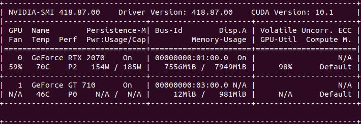
As I stated earlier, one of the nice things about running training locally was getting to see the resource utilization up close. This what a snapshot of that looks like:

Not to mention that long hours of training provided decent heating for the starting Winter season, much to the detriment of my electric bill.

In the next post, I’ll describe my experiments with a convolutional neural work trained from scratch and a transfer learning supported model.