In this mini-series of posts, I will describe a hyper-parameter tuning experiment on the fashion-mnist dataset.
I wanted to test out a guided and easy way to run hyper-parameter tuning. In Part II, I described setting up the end-to-end pipeline with a baseline, and running hyper-parameter tuning with the hyperopt package. In this third and final chapter, I describe my target models, a convolutional neural network trained from scratch and a transfer learning model.
Much has already been written about the inner workings, theoretical understanding - or lack of -, as well as the conspicuacies of training convolutional neural networks. To me, one of the most useful articles in this space is Karpathy’s CS231 Convolutional Neural Networks for Visual Recognition.
In this post, I’ll briefly discuss the architectural design of the networks I trained, tuning parameters, and my observations from experimental runs.
The Architecture
I was curious to try out transfer learning for this problem. I had trained convolutional networks on problems before, so transfer learning posed more of a novelty to me. However, it felt incomplete to look at benchmarks for the baseline against a transfer learning model without knowing what training a convolutional network from scratch would do.
Thus, I decided to do both. Train a convolutional network from scratch. And use an existing model for transfer learning. For both cases, I had to make some artchitectural choices. There are some well known network architectures out there, like the Inception and ResNet. Discussing these architectures is a topic that merits its own post.
I elected to implement a VGGNet inspired network and to use VGG19 model trained on imagenet for the transfer learning task.
ConvStrix: Vanilla Model
In this architecture, there are blocks of layers connected. Each block is made up of one or more 2D convolutional layers (3x3). Every block, with the exception of the last one, is followed by a layer of batch normalization prior to max-pooling (2x2). And with each block, the number of filters is incremented by a multiple the initial value of 32.
The final block is followed by one or more fully connected layers, each with dropout, ending with the final layer of labels.
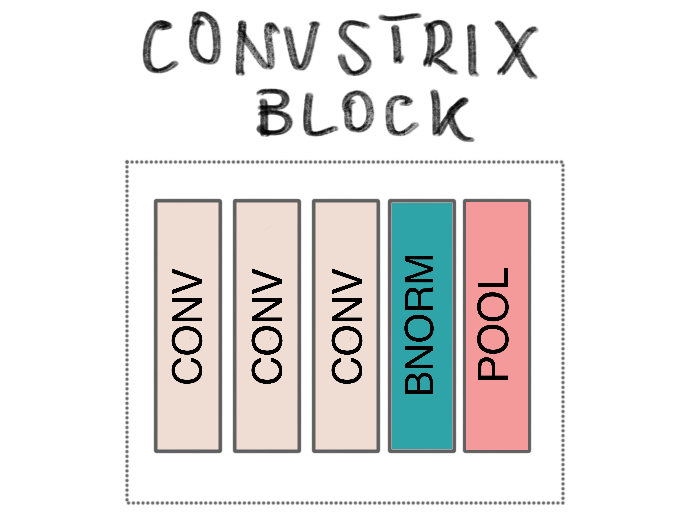
I named the architecture ConvStrix, and it’s a relatively straightforward design, but it allowed the observation of certain behaviours with regards to parameters. For instance, since the kernel sizes are the same, input reduction after each block followed a fairly linear pattern. This also simplified reasoning about hyper-parameter search spaces, which was my main intent.
VGGStrix: Transfer Learning Model
This model had a very similar architecture to ConvStrix, with one exception: the first “block” was the entire sequence of convolutional blocks on the VGG19 network.
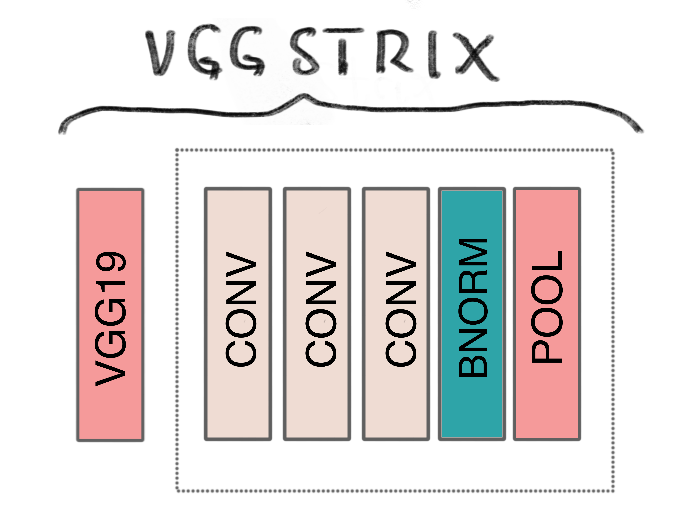
Loading a pre-trained model with tensorflow keras was relatively straightforward. With the VGGStrix model, one question I grappled with was whether I should make the final layers of the VGG19 network trainable or add convolutional layers to it. I went with the latter, because I wanted to add convolutional blocks to reduce the size of the output anyways. I did make the number of convolutional blocks a parameter, so that during tuning, a design without any could be tested.
Let’s turn to the hyper-paramater search space definition.
Tuning
Similar to how I specified a hyper-search-space for the baseline model, I did the same for ConvStrix and VGGStrix.
ConvStrix
{
  'batch_size': hp.choice('batch_size', options=[2 ** x for x in range(4, 6 + 1)]),
  'learning_rate': hp.loguniform('learning_rate', low=np.log(0.0001), high=np.log(1)),
  'num_blocks': scope.int(hp.quniform('num_blocks', low=2, high=6, q=1)),
  'block_size': scope.int(hp.quniform('block_size', low=1, high=3, q=1)),
  'fcl_num_layers': scope.int(hp.quniform('fcl_num_layers', low=1, high=4, q=1)),
  'fcl_layer_size': hp.choice('fcl_layer_size', options=[512, 768, 1024, 1536]),
  'fcl_dropout_rate': hp.quniform('fcl_dropout_rate', low=0.05, high=0.5, q=0.05),
  'activation': hp.choice('activation', options=['relu', 'selu', 'tanh']),
  'optimizer': hp.choice('optimizer', options=['adam', 'adamax', 'nadam', 'rms-prop'])
}
The fcl_ prefixed parameters refer to the fully connected block. As with the baseline, I experimented with training parameters such as batch size, and optimizer. For the convolutioal blocks, I experimented with their count and size, which was uniform for each block. I did, once again, refrain from experimenting with nested parameters (e.g. number of convolutional layers per block).
VGGStrix
{
  'batch_size': hp.choice('batch_size', options=[2 ** x for x in range(4, 6 + 1)]),
  'learning_rate': hp.loguniform('learning_rate', low=np.log(0.0001), high=np.log(1)),
  'conv': hp.choice('conv', [
      {'num_blocks': 0, 'block_size': 0},
      {'num_blocks': 1, 'block_size': scope.int(hp.quniform('block_size', low=1, high=3, q=1))},
      {'num_blocks': scope.int(hp.quniform('num_blocks', low=2, high=3, q=1)), 'block_size': 1}
  ]),
  'fcl_num_layers': scope.int(hp.quniform('fcl_num_layers', low=1, high=4, q=1)),
  'fcl_layer_size': hp.choice('fcl_layer_size', options=[512, 768, 1024, 1536]),
  'fcl_dropout_rate': hp.quniform('fcl_dropout_rate', low=0.05, high=0.5, q=0.05),
  'activation': hp.choice('activation', options=['relu', 'selu', 'tanh']),
  'optimizer': hp.choice('optimizer', options=['adam', 'adamax', 'nadam', 'rms-prop'])
}
Because the models have very little distinction in terms of their architecture, the hyper-paramaters are the same, with one minor exception: this time, I added conditional branches to the search tree. See, the output of the VGG19 network can only be convolved so many times with my chosen kernel size. Three times to be exact. And I wanted to test a network without any convolutional blocks. Thus, I created a sub-tree that partitions the the number of blocks into three ranges: none, one containing [1, 3] layers, and [2, 3] with exactly one layer. This was to prevent invalid combinations, which would only waste resources.
Now we can address some issues encountered during training and paramater exploration.
Computing
Convolutional networks can take up… a lot… of memory! Lots. And lots. Of Memory.
Generally, for an architecture like the VGG19, this memory hog is concentrated on the final layer, where the output of the last convolutional block connect with a fully connected layer. Thus, the following holds: the smaller the final output, the less paramaters there will be. Fewer parameters can be achieved with either aggresive or more convolution. From experiments, it holds that more layers work better. Thus, rather than being aggresive, I opted to increase the number of layers, and reduce the size of the output of each progressively.
However, more layers means more paramaters. Generally speaking though, these tend to be inconsequential compared to the number of paramaters that go into fully connected layers. Still, having many of these convolutional blocks take up memory. And depending on the optimizer you use, each one may require three to four times the number of values to compute back-propagation. And this number if multiplied by the number of images in a batch.
On my computer, I couldn’t run more than one VGGStrix model at any given time. With ConvStrix, I could.
I still wanted to reduce the total runtime of the experiment as much as possible, prevent resource waste, so I implemented early stopping with a patience of 5 - i.e. if the validation loss does not improve in 5 epochs, training stops, and the best parameters so far are restored to be exported.
Results
I ran 50 trials for ConvStrix, the vanilla convolutional neural network, and 50 trials for VGGStrix, the transfer learning model with VGG19. I did not record the wall clock time for the ConvStrix experiment, but I did for the VGGStrix, and it was about 15 hours. Recall that the former could use parallelism while the latter could not - due to resource constraints. I did not use early stopping when doing a final run with the best parameters.
ConvStrix
The top results from the experiment are listed below. Unlike the baseline feed forward neural work, different combinations of parameters seemed to work well together for this model. In general, having more single convoluational blocks worked better, i.e. depth proved to be relevant for this problem, in line with other reported results.
Performance on the test set was relatively superior to that of the baseline model, with 94% accuracy - 9 percentage points (pp) higher.
                 precision    recall  f1-score   support

t-shirt-or-top      0.877     0.895     0.886      1000
       trouser      0.984     0.995     0.990      1000
      pullover      0.915     0.901     0.908      1000
         dress      0.923     0.951     0.937      1000
          coat      0.900     0.925     0.912      1000
       sandals      0.993     0.985     0.989      1000
         shirt      0.838     0.774     0.805      1000
       sneaker      0.967     0.975     0.971      1000
           bag      0.988     0.986     0.987      1000
   ankle-boost      0.974     0.978     0.976      1000

      accuracy                          0.936     10000
     macro avg      0.936     0.936     0.936     10000
  weighted avg      0.936     0.936     0.936     10000
VGGStrix
A listing of the top results for VGGStrix is given below. Like ConvStrix, different combinations of parameters worked well. Noticeably, having no convolutional blocks after VGG19 worked better.
Performance of this model was also higher than that of the baseline, but fell short compared to the vanilla model by ~1.7pp.
                 precision    recall  f1-score   support

t-shirt-or-top      0.845     0.897     0.870      1000
       trouser      0.993     0.990     0.991      1000
      pullover      0.842     0.898     0.869      1000
         dress      0.922     0.937     0.930      1000
          coat      0.888     0.859     0.873      1000
       sandals      0.976     0.978     0.977      1000
         shirt      0.822     0.719     0.767      1000
       sneaker      0.952     0.962     0.957      1000
           bag      0.976     0.992     0.984      1000
   ankle-boost      0.973     0.962     0.967      1000

      accuracy                          0.919     10000
     macro avg      0.919     0.919     0.919     10000
  weighted avg      0.919     0.919     0.919     10000
Conclusions
In the end, we found that ConvStrix, a VGG inspired network trained from scratch, performend best. Given the margin of performance difference within each possible architecture, and across models, hyper-parameter tuning proved highly useful for achieving really good performance. More can be said about the computational cost for hyper-parameter tuning, of course. This problem involved a relatively simple dataset and non-industrial grade compute resources. Still, the number of epochs needed for each execution to reach a satisfactory level of performance was relatively acceptable. I believe that sampling and small epochs can be sufficient to identify the best candidates for a full scale training - for instance, most experiments in the VGGStrix didn’t make it to their 20th epoch before early stopping kicked in.
It was interesting for me to observe disparate combinations of parameters working well for the convolution based models, while there was pretty much a uniform set of parameters that did so for the feed forward neural network. Given the long run time and computational demands of the experiments - and slugishness of the user experience I faced on my desktop during training - I think it’s safe to say it’s best to delegate such trials to a cloud environment. I do believe there is immense value in having local resources for testing and debugging though.
My key takeaways were:
- Setting up and configuring local runtime environments can be troublesome (tensorflow, CUDA, cuDNN…), but provides valuable fast feedback loops in the long run.
- It’s relatively easy to entrust smart algorithms encoded in practical libraries to tune parameters in models with very low overhead - in this case, with hyperopt
- Analyzing the results of different experiments can yield intuitions on what works - at least, for the dataset in hand.
- Gaming GPUs are great… but not that powerful in practice for deep learning.
- Shirts on this dataset are apperantly harder to classify than any other clothing item
I didn’t get a result higher than the highest reported on the fashion-mnist leaderboard. There is obvisouly more that can be done - e.g. data augmentation, stacked models. We leave those challenges for a different time.